Lyapunov stability of a linear PDE
Consider the partial differential equation (PDE)
subject to the boundary conditions \(u(0)=0=u(1)\).
In this example we use QUINOPT to find a polynomial \(p(x)\) of degree 4 such that the functional
is a Lyapunov function proving the global stability of the zero solution \(u(x)=0\) when \(k=15\). This means that we must find \(p(x)\) such that, for some constant \(c>0\),
Note that since both inequalities are homogeneous in \(p(x)\), we may without loss of generality take \(c=1\).
Download the MATLAB file for this example
1. Set up the variables
As usual, we start by cleaning up from previous work and defining the basic problem variables:
>> clear
>> yalmip clear
>> quinopt clear
>> x = indvar(0,1);
>> u = depvar(x);
Then, we set up the PDE:
>> k = 15;
>> u_t = u(x,2) + (k-24*x+24*x^2)*u(x);     % the right-hand side of the PDE
>> bc = [u(0), u(1)];                       % the boundary conditions
Finally, we define the polynomial p(x), the coefficients of which are the optimization variable. We use the command legpoly() to define a polynomial with variable coefficients in the Legendre basis (this is convenient because QUINOPT represents the variables with Legendre series expansions internally):
>> p = legpoly(x,4); % Create the variable polynomial p(x)
Note
The coefficients of \(p(x)\) can be obtained using the commandcoefficients():
>> c = coefficients(p); % c is a vector containing the variable Legendre coefficients of p
or, more simply, by using two outputs when creating \(p(x)\) with the command legpoly()
>> [p,c] = legpoly(x,4); % c is a vector containing the variable Legendre coefficients of p
2. Set up & solve the integral inequalities
To set up the inequalities in QUINOPT, simply specify their integrands as the elements of a vector EXPR:
>> EXPR(1) = (p-1)*u(x)^2;              % \int p(x)*u(x)^2 >= \int u(x)^2
>> EXPR(2) = -2*p*u(x)*u_t;             % -V_t(u) >=0.
To solve for p(x) and obtain some information about the solution, we use the command quinopt() with one output argument:
>> SOL = quinopt(EXPR,bc);
The output SOL contains information about the solution, such as the CPU time taken to set up and solve the problem. In particular,the field SOL.FeasCode indicates whether the problem was solved successfully (in this case, SOL.FeasCode==0). For more information on QUINOPT’s outputs and the meaning of feasibility codes, check
>> help quinopt
>> quinoptFeasCode
Note
It may be shown that the PDE we are analysing is unstable if \(k=16\). In this case, no suitable polynomial \(p(x)\) exists, and the feasibility problem solved by QUINOPT is infeasible. This can be verified by checking the value of SOL.FeasCode.
4. Plot \(p(x)\)
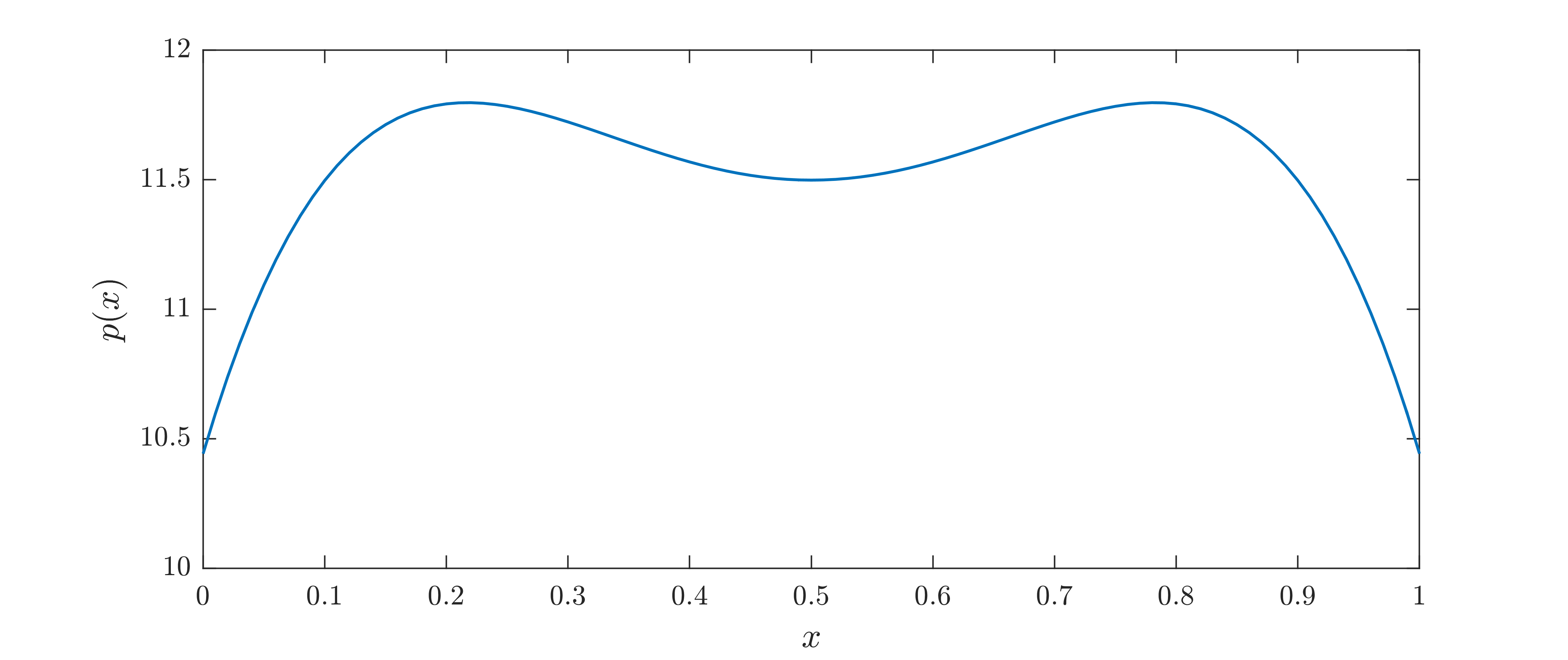
Once a feasible polynomial \(p(x)\) is found, as is the case when \(k=15\), one may wish to see what it looks like. MATLAB’s usual plot() function is overloaded on polynomials defined with the command legpoly(), making it really easy to plot \(p(x)\). Juse type:
>> xval = 0:0.01:1;          % the values of x at which p is plotted
>> plot(xval,p)
An example of what \(p(x)\) might look like is shown below.
Important
When using plot() on a Legendre polynomial variable, the values xval must within the domain of the independent variable x originally used to define the polynomial. Otherwise, plot() throws an error. The function getDomain() can be used to check the domain over which a Legendre polynomial is defined.